Data Tables
This exercise will teach you how to build your own customized 3-year data tables full of stats for NFL's top QB's, RB's, WR's, and TE's.
The first section demonstrates the step-by-step process to build the QB table, and then the same table will be used for the RB, WR, and TE tables with just a couple clicks. This is just a starting point. Feel free to expand to other stats, seasons, players, etc.
Let's start by creating a Pivot table which is covered here in our Microsoft Excel Tools section where you can learn more about building pivot tables, and how to apply other functions and formats to really start creating your own in-depth analysis.
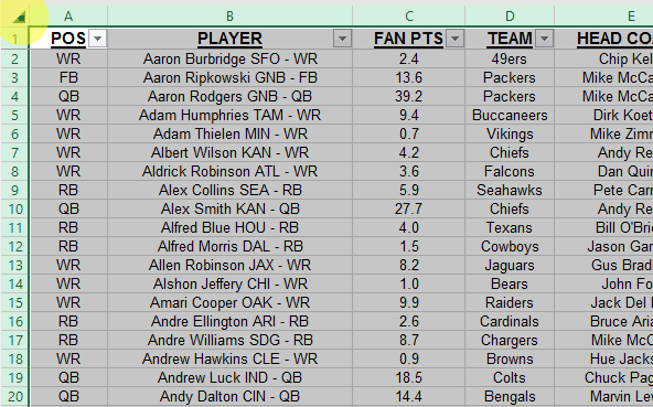
First let's select all of our data by clicking the box in the top left corner by Column A and Row 1.
Choose the Insert Menu.
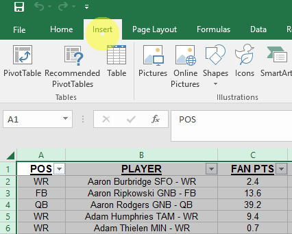
Select Pivot Table.

Make sure our entire range of data is selected. In this case it's Column A to Column AJ.
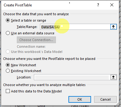
Now let's created this Pivot Table in a New Worksheet, and click OK.

Click anywhere in the Pivot Table on the left to open the Pivot Table Fields on the right.

In the Pivot Table Fields on the right, drag Pos in the top list down to Filters so that we can quickly change from QB to RB, WR, and TE. Now let's add the Player field from the top list down to the Rows section

Now drag Season to the Columns section, and drag Fan Pts down to Values. Make sure that the field is set to Sum because we want to see each players total fantasy points for each season.

Now let's also add Passing Yards from the top list to the Values section along with Fantasy Points. Notice now a Values field appears in the Columns section below Season.

This means that our Pivot table will show all of our Values (in this case we have Fantasy Points and Passing Yards) under each Season.

We want to see each Season together for each value (Fantasy Points and Passing Yards), so let's drag Values above Season in the Columns section.

Now you can see each players total fantasy points for each season, and then their total passing yards for each season.

Now let's add Passing Touchdowns and Interceptions to our values, and make sure that we are doing a sum of those as well.

Over to the left where our Pivot Table is forming, you can see data from all of the seasons going back to 2000, and the seasons are listed from smallest to largest. Click the Column Labels arrow, and only select season 2014, 2015, and 2016.

Let's also sort the seasons from Largest to Smallest. If you see Sort Z to A, this works as well.

Right-click anywhere in the 2016 Fantasy points column (column B in this case), and sort from Largest to Smallest so that our lists starts with the top fantasy performers for 2016.

Now let's click on the position filter that we created at the top.

You may need to check the box on the bottom that says Select Multiple Items.

Let's filter to only QB's.

Now our table is getting somewhere.

You can always copy any data that you want, and paste it somewhere else to work on outside of the Pivot Table. In this case, we're going to select just the top 20 players. Make sure to include all of our values (Fantasy Points, Passing Yards, Passing TD's, and Interceptions) in your selection.

Let's paste this data over to the right in cell T1.

You can see our data gets cut off because the columns are too skinny. If you double-click on the dividing line in between 2 columns at the top, the column will expand accordingly.

If you have multiple columns selected, they will all adjust by just clicking any divider within the selection.

Let's change "Row Labels" above our players in cell T2 to Players.

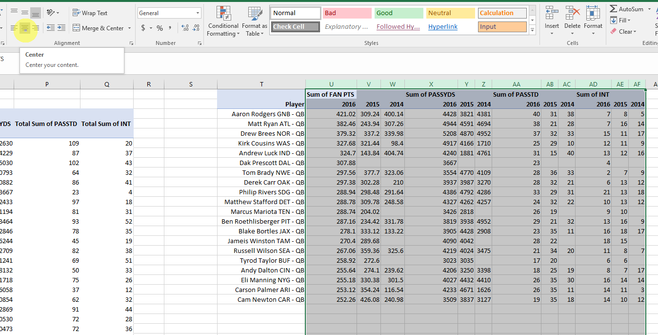
Now we're going to select column T, and align it to the right side. This is found in the Home menu.

Let's also center the rest of the columns. Select column U to column AF, and click the center alignment button.
Now we're going to merge some cells to make this look better. Select cell U1 where it says "Sum of FAN PTS", and also highlight cells V1 and W1 along with it.

Now that we have cells U1:W1 selected, click on the Merge & Center button.

This merges and centers our fantasy points title above all 3 years.

Let's do the same for the other categories. Once you merge the cells, let's change the names from Sum of Fan PTS, Sum of PASSYDS, Sum of PASSTDS, and Sum of INT to: Fantasy Points, Passing Yards, Passing TD's, and Interceptions.

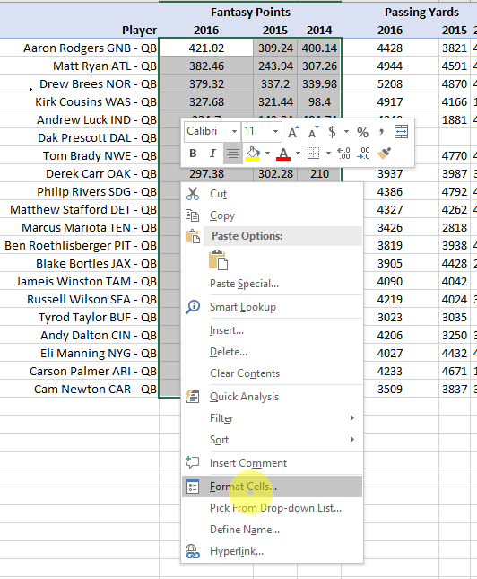
Let's select our fantasy points (cells U3:W22) for formatting. You can format any cells by right-clicking on them, and selecting Format Cells...
Let's change our fantasy points to number values.

We'll also change the decimal places to 1.

That looks much cleaner.

Let's highlight Passing Yards in cells X2:Z22. Right-click, Format Cells, and let's add the comma since our values will definitely go over 1,000.

It will look better if we adjust our columns to the same width. Select columns U:W. Click and hold any divider between the letters at the top of the columns. Drag right or left to resize, and the other columns will automatically adjust to the same width. This also works up and down with rows.

Apply the same adjustments to the column widths for Passing Yards, Passing TD's, and Interceptions.

We are almost there, but let's make this table look even better. Select everything (T1:AF22), and let's add some borders. The borders menu can be found close to the alignment buttons.

Let's select All Borders. This will thinly outline every cell in our selection.

Now we can add a thicker border around each section to break them up a bit. Select T1:T22 and apply the Thick Outside Border.

Apply the same thick border to the other sections:
Fantasy Points - U1:W22
Passing Yards - X1:Z22
Passing TD's - AA1:AC22
Interceptions - AD1:AF22
Also put the thick border around cells T1:AF2 to separate the titles from the data.

The final touch will be to simply Merge & Center cells T1:T2 above the players.

That's it! I moved everything down 1 row, and added a title for our table by merging & centering the cells.

Great job!
Make sure to save the QB table somewhere else so that you can use this as a template to quickly create the other tables.
Not only have we engineered a pretty slick table of QB stats, we've also built the foundation where we're going to quickly and easily create our RB, WR, and TE tables.
Go back to the Pivot Table, and change the Position Filter up at the top left from QB to RB.

We are now looking at just RB's, so let's go over to our Pivot Table Fields on the right (click anywhere in the Pivot Table to make the Pivot Table Fields appear), and get rid of the Passing Yards, Passing TD's, and Interceptions in the Values section. You can click on them and select Remove Field, or simply drag them back up to the main list at the top.

Add Rushing Attempts, Rushing Yards, and Rushing TD's. Make sure they are all set to Sum.

We still have the same layout that we created for our QB table, so just select and copy the top 20 players, and their stats.

We are going to paste the new RB data where we have Aaron Rodgers in the table that we've created for the QB's, but we do not want to lose any of the formats that we've set up. Instead of a regular paste, right-click, select Paste Special, and select Values. (You can also just click the clipboard with the 3 little numbers above the Paste Special option to only paste values)

Don't forget to change the main title from QB to RB. Also change the categories from Passing Yards, Passing TD's, and Interceptions, to Rushing Attempts, Rushing Yards, and Rushing TD's.

We now have Yards where we previously had TD's, so let's select and format these values.

Make sure that the Category is set to Number, and we're looking at yards now instead of TD's, so let's add the comma for anything over 1,000.

See how easy that was! Again, make sure to save this RB table somewhere else so that you can keep using this table as a template to quickly create the other tables.

Of course the same process applies to WR's. Select WR instead of RB in the Position filter in the top left corner.

Remove Rushing Attempts, Rushing Yards, and Rushing TD's.

Add Targets, Receiving Yards, and Receiving TD's to the Values.

Copy the WR data.

Using Paste Special, paste only the values into the previously created table.

Change the title names:
RB to WR
Rushing Attempts to Targets
Rushing Yards to Receiving Yards
Rushing TD's to Receiving TD's

WR Stats Table complete. Save and move on.

For the TE's, you guessed it. Simply change the Position filter from WR to TE.

Copy the TE data.

Paste only the values with Paste Special.

All of the categories are the same for TE's, so the only name that needs to be changed is the main title. Simply change WR to TE.

4 clean and formatted Stat tables just like that!
